CryptoDataPy

CryptoDataPy allows you to create high quality ready-for-analysis data sets from a variety of sources with only a few lines of code. The easy to use interface facilitates each step of the ETL (extract-transform-load) process, saving you from having to spend countless hours studying documentation, extracting data from different file formats and sources, as well as wrangling and cleaning the data.

In this notebook, we will walk through how to use CryptoDataPy to collect various types of data from multiple sources and get it ready for data analysis.

Quick Start:

• Long/short strategies: perpetual futures prices for long/short algo trading strategy development, with sample history extended back using aggregate exchange spot prices.

• Data cleaning: on-chain data cleaning in a few lines of code.

• Stablecoin analysis: key indicators for the largest stablecoins.

Objects:

• DataCatalog allows you to explore what data is available and understand it better.

• DataRequest provides an intuitive interface which allows you to specify the parameter values for the data you want.

• GetData retrieves either metadata or time series data from the data source for the parameters specified in the data request.

• CleanData provides tools for data cleaning: filtering and repairing outliers, filtering assets trading below an average traded value (liquidity), removing observations with long periods of missing values, removing tickers with short price histories (minimum number of observations), and removing tickers to be excluded from the analysis (e.g. stablecoins).

Long/Short Strategies

Let’s collect market and funding rate data for long/short algo trading strategy research.

import pandas as pd
from matplotlib import pyplot as plt
import warnings
warnings.filterwarnings("ignore")

---------------------------------------------------------------------------
ModuleNotFoundError                       Traceback (most recent call last)
Cell In[1], line 1
----> 1 import pandas as pd
      2 from matplotlib import pyplot as plt
      3 import warnings

ModuleNotFoundError: No module named 'pandas'

Step 1: Define Asset Universe

First, we need to import DataRequest and GetData which will allow us to create a tickers list for our asset universe.

from cryptodatapy.extract.datarequest import DataRequest
from cryptodatapy.extract.getdata import GetData

Let’s get a list of tickers for the universe of assets with perpetual futures contracts trading on binance, the most liquid cryptoasset exchange.

data_req = DataRequest(source='ccxt')
perp_tickers = GetData(data_req).get_meta(method='get_markets_info', exch='binanceusdm', as_list=True)

Which gives us an asset universe of 150 + cryptoassets.

len(perp_tickers)

191

Step 2: Get Perpetual Futures Data

Next, let’s create a data request for both market prices and funding rates for those perpetual futures tickers, using only the first 10 tickers for illustrative purposes.

Note: using the source_tickers parameter is recommended when the tickers are already in the data source’s format. If data source’s format is not known, CryptoDataPy will convert tickers to source tickers automatically.

data_req = DataRequest(source='ccxt',
                       source_tickers=perp_tickers[:10], 
                       fields=['close', 'volume', 'funding_rate'], 
                       mkt_type='perpetual_future', 
                       freq='d')

We can now retrieve this data request using the GetData object and the get_series method.

df = GetData(data_req).get_series()

df.head()

		close	volume	funding_rate
date	ticker
2019-09-08	BTC	10391.63	3096.291	<NA>
2019-09-09	BTC	10307.0	14824.373	<NA>
2019-09-10	BTC	10102.02	9068.955	<NA>
2019-09-11	BTC	10159.55	10897.922	0.0003
2019-09-12	BTC	10415.13	15609.634	0.0003

Step 3: Extend Sample Size with Spot Data

Since perpetual futures only started trading in 2019 on Binance, this gives us a limited sample size for quantitative research. Let’s extend it back using spot prices from another data source.

We will need to replace the market tickers with base asset tickers first from aggregate exchange prices on CryptoCompare before pulling the data.

cc_tickers = [ticker.split('/')[0] for ticker in perp_tickers]

data_req = DataRequest(source='cryptocompare',
                       tickers=cc_tickers[:10], 
                       fields=['close', 'volume'], 
                       mkt_type='spot', 
                       freq='d')

df1 = GetData(data_req).get_series()

We can now combine the two datasets to extend our history back to 2010.

df = df.unstack().combine_first(df1.unstack()).stack()

df.head()

		close	funding_rate	volume
date	ticker
2010-07-17	BTC	0.04951	<NA>	20.0
2010-07-18	BTC	0.08584	<NA>	75.01
2010-07-19	BTC	0.0808	<NA>	574.0
2010-07-20	BTC	0.07474	<NA>	262.0
2010-07-21	BTC	0.07921	<NA>	575.0

Step 4: Filter Asset Universe

Lastly, we may want to filter this asset universe by:

• identifying and repairing outliers

• removing low trading volume cryptoassets (< $10 mil USD average traded volume)

• removing cryptoassets with a limited data history (< 100 observations)

We will need to import CleanData to use the filter methods available.

# import CleanData 
from cryptodatapy.transform.clean import CleanData

ERROR:prophet.plot:Importing plotly failed. Interactive plots will not work.

# Filter data
clean_df = CleanData(df).filter_outliers(od_method='mad').\
                         repair_outliers(imp_method='interpolate').\
                         filter_avg_trading_val(thresh_val=10000000).\
                         filter_missing_vals_gaps().\
                         filter_min_nobs().get(attr='df')

clean_df.dropna(how='all').head()

		close	funding_rate	volume
date	ticker
2014-12-09	BTC	352.19	<NA>	43827.16
2014-12-10	BTC	347.94	<NA>	27133.46
2014-12-11	BTC	347.68	<NA>	51080.97
2014-12-12	BTC	353.4	<NA>	26850.92
2014-12-17	BTC	320.02	<NA>	61338.52

We have extended our data sample by an extra 5 years and are now ready to do some long/short algo trading strategy research!

Data Cleaning

Cryptoassets create a lot of data, but the data can have a lot of outliers and irregularities that can wreak havoc with predictive/ML models down stream. This is especially true for on-chain data and off-chain data, as well as higher frequency market data.

This makes data cleaning and important part of any high quality cryptoasset data pipeline.

Step 1: Data Extraction

Let’s start by collecting our data.

# glassnode
data_req = DataRequest(source='glassnode', 
                       tickers=['btc', 'eth'], 
                       fields=['close', 'add_act', 'hashrate'], 
                       freq='d',
                      start_date='2016-01-01')

df = GetData(data_req).get_series()

With same data request parameters, can you retrieve the same data from other sources for comparison.

# coinmetrics
data_req = DataRequest(source='coinmetrics', 
                       tickers=['btc', 'eth'], 
                       fields=['close', 'add_act', 'hashrate'], 
                       freq='d',
                      start_date='2016-01-01')
df1 = GetData(data_req).get_series()

# cryptocompare
data_req = DataRequest(source='cryptocompare', 
                       tickers=['btc', 'eth'], 
                       fields=['close', 'add_act', 'hashrate'], 
                       freq='d',
                      start_date='2016-01-01')
df2 = GetData(data_req).get_series()

Step 2: Visual Data Inspection

Next, we can plot the series from various sources to compare them.

# concat dfs
df3 = pd.concat([df, df1, df2], axis=1)
add_act_df = df3.loc[pd.IndexSlice[:, 'ETH'], 'add_act'].droplevel(1)
# rename cols
col_names = [vendor + '_' + 'ETH_' + 'active_addresses' for vendor in ['glassnode', 'coinmetrics', 'cryptocompare']]
add_act_df.columns = col_names
# plot active addresses
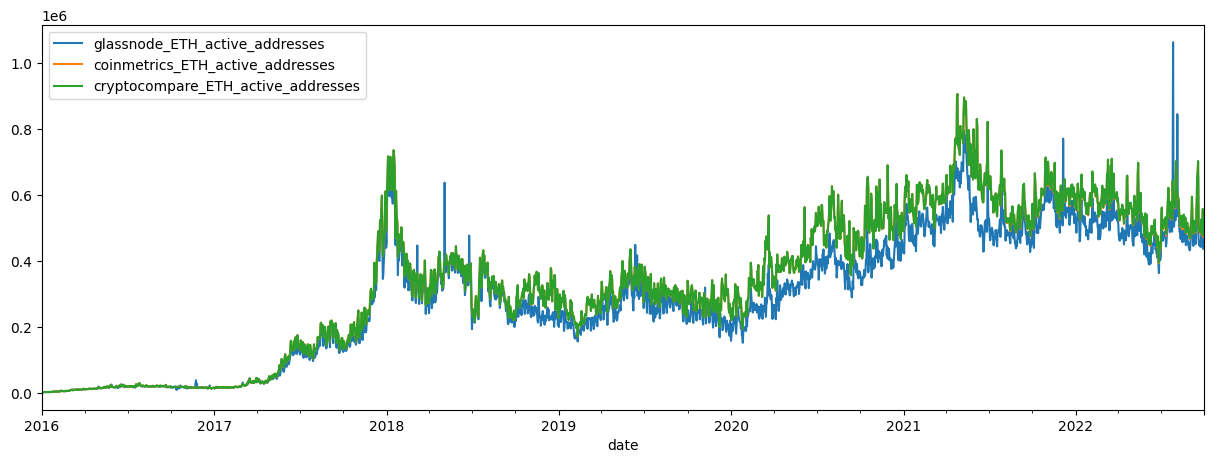
add_act_df.plot(figsize=(15,5))
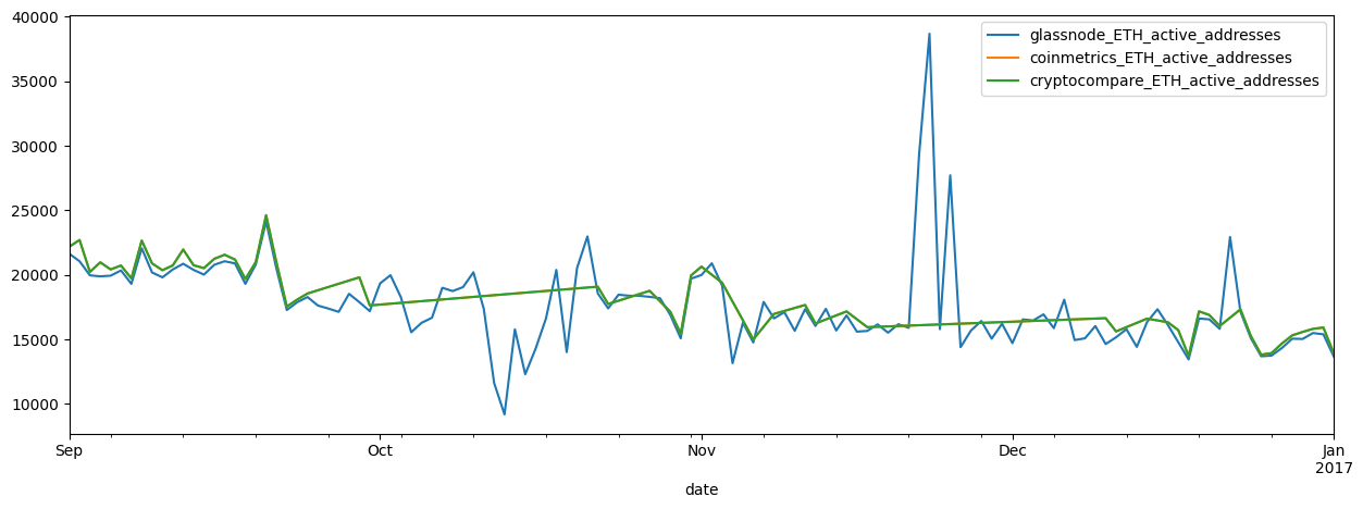
add_act_df.loc['2016-09-01':'2017-01-01'].plot(figsize=(15,5))
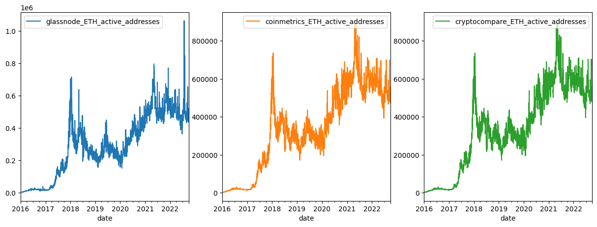
add_act_df.plot(subplots=True, layout=(1,3), figsize=(15,5))
plt.legend(loc='upper right');

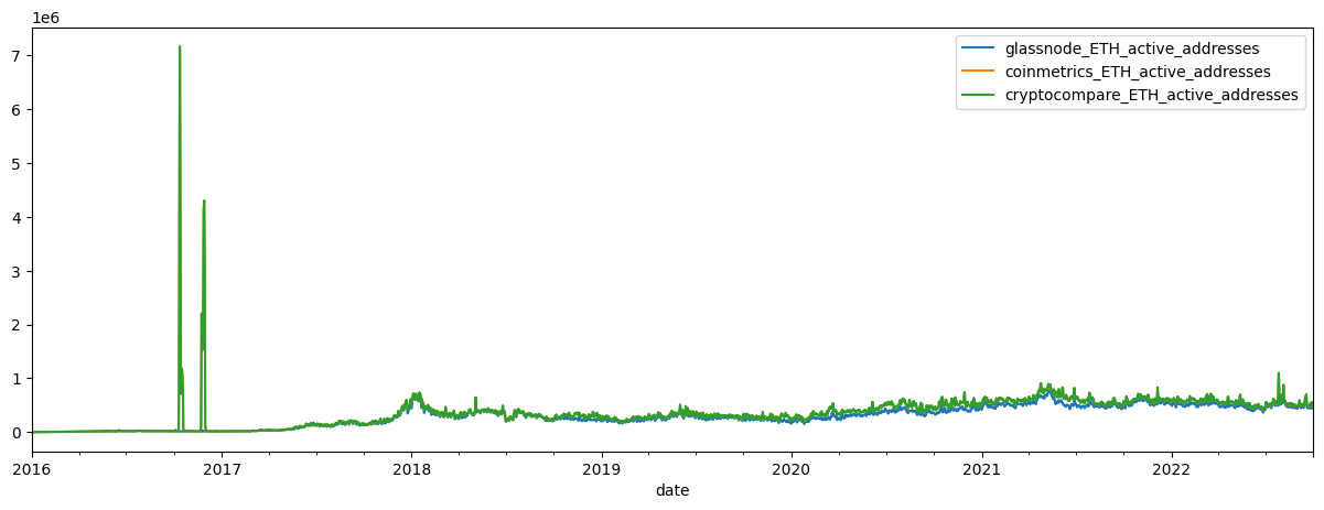
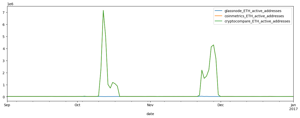
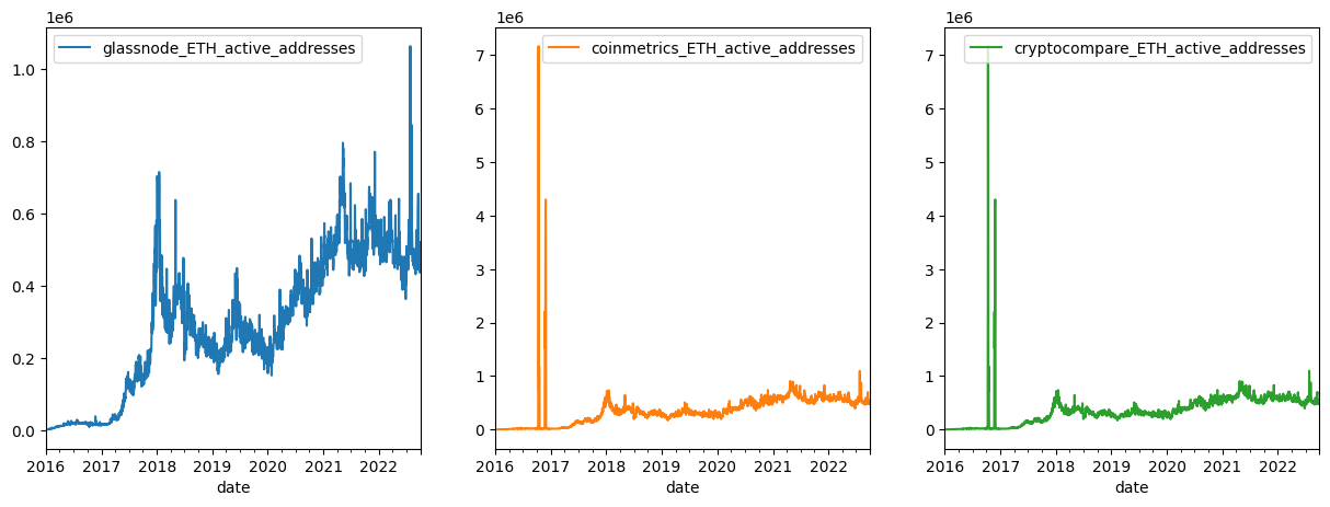
Comparing the three active address series, we notice that both the Cryptocompare and Coinmetrics active addresses appear to have large outliers in ETH active addresses in late 2016.

Large outliers can cause major distortions down stream in any machine learning or predictive process so cleaning this data before doing so is a necessary next step.

Step 3: Data Cleaning

Once outliers are detected through visual data inspection, they can be filtered and repaired by importing CryptoDataPy’s CleanData module.

We have several options:

1. Use the series without large outliers.

2. Filter the outliers using one of CryptoDataPy’s outlier detection methods (shown below) and keeping the ‘clean’ series.

3. Combine 1 and 2, e.g. filtering and repairing outliers using outlier detection and missing values imputation algorithms, and then taking the median (or some other measure of central tendency) from the resulting series as the representative ‘true series (also shown below).

# import CleanData
from cryptodatapy.transform.clean import CleanData

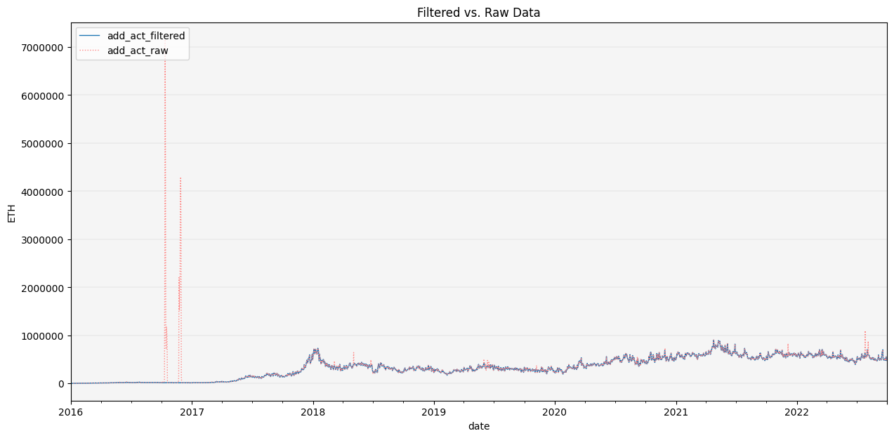
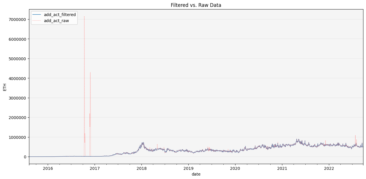
Here, we will use the STL outlier detection algorithm, similar to the one used by Twitter to filter/remove outliers, and then use the interpolation method for outlier repair.

# filter cryptocompare data 
# show raw vs filtered plot
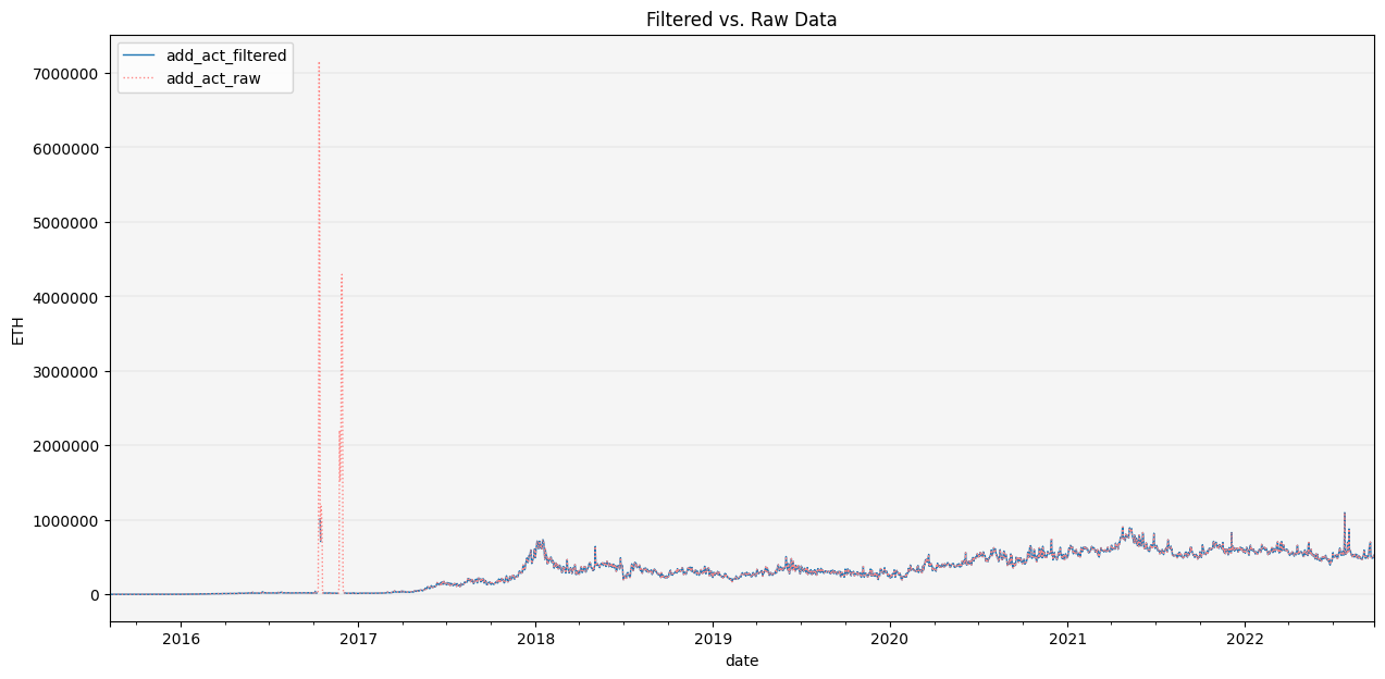
CleanData(df2).filter_outliers(od_method='stl').\
               repair_outliers(imp_method='interpolate').\
               show_plot(plot_series=('ETH', 'add_act'))
# save filtered df
clean_df2 = CleanData(df2).filter_outliers(od_method='stl').\
                           repair_outliers(imp_method='interpolate').\
                           get(attr='df')

Let’s visually inspect the data once again to assess data quality.

# concat dfs
df_clean = pd.concat([df, clean_df1, clean_df2], axis=1)
add_act_df1 = df_clean.loc[pd.IndexSlice[:, 'ETH'], 'add_act'].droplevel(1)
# rename cols
col_names = [vendor + '_' + 'ETH_' + 'active_addresses' for vendor in ['glassnode', 'coinmetrics', 'cryptocompare']]
add_act_df1.columns = col_names
# plot active addresses
add_act_df1.plot(figsize=(15,5))
add_act_df1.loc['2016-09-01':'2017-01-01'].plot(figsize=(15,5))
add_act_df1.plot(subplots=True, layout=(1,3), figsize=(15,5))
plt.legend(loc='upper right');

These data cleaning algorithms do a good job of filtering and repairing large outliers as we can see.

We can now use one of the ‘cleaned’ data sets for data analysis, or alternatively, use all 3 series to construct a ‘series of truth’ which uses the median of the 3 time series.

# plot series of truth
df_clean.add_act.median(axis=1).unstack()['ETH'].plot(title='ETH Active Addresses - Series of Truth', figsize=(15,7));

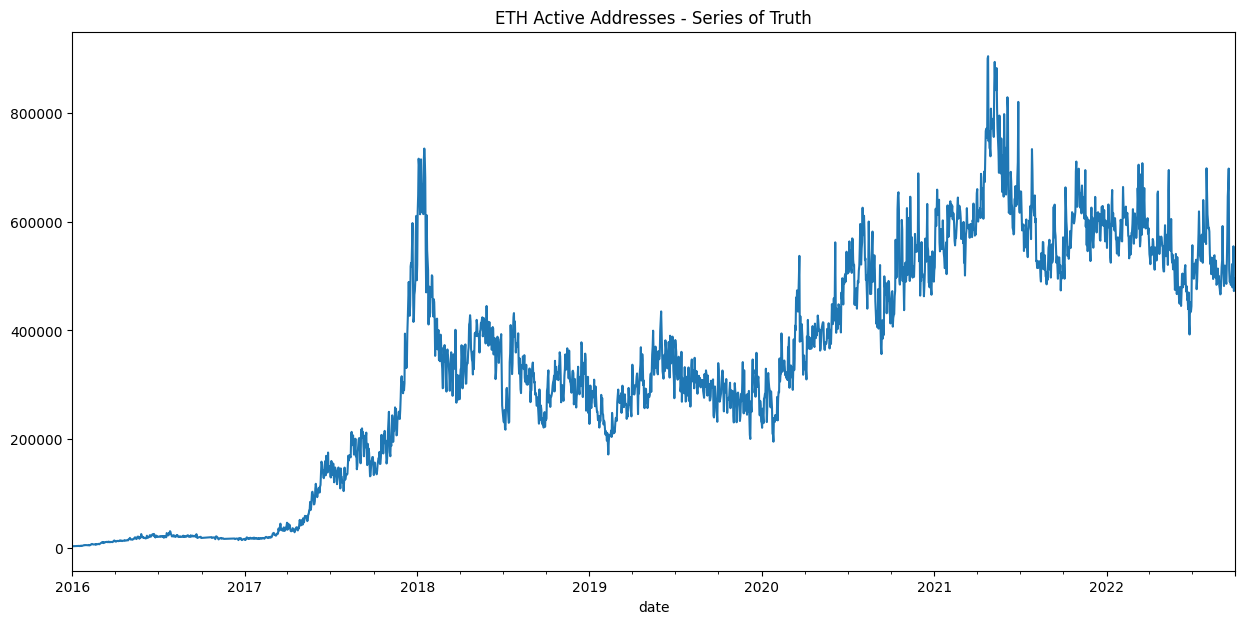
You are now ready to begin exploring, analyzing and predicting with clean data!

Stablecoin Analysis

Stablecoins are a growing and import part of the cryptoeconomic ecosystem. The recent failures of some stablecoin projects and the broader impact this can have on the ecosystem makes risk monitoring and analysis of stablecoins increasingly import.

CrptoDataPy makes it easy to find data on stablecoins.

The DataCatalog allows us to find information on the largest stablecoins by market cap.

from cryptodatapy.util.datacatalog import DataCatalog 
dc = DataCatalog()

If we want to get metadata

sc_meta = dc.get_tickers_metadata(cat='crypto')

sc_meta.head()

	name	description	url	country_id_2	country_id_3	country_name	agg	category	subcategory	mkt_type	frequency	tenor	unit	quote_ccy	tiingo_id	fred_id	dbnomics_id	investpy_id
ticker
USDT	Tether USDT	USDT is a cryptocurrency asset issued on the B...	NaN	WL	WLD	World	WL	crypto	stablecoin	spot	tick	NaN	fiat currency per unit of stablecoin	NaN	NaN	NaN	NaN	NaN
USDC	USD Coin	USD Coin (USDC) is a fully collateralized US ...	NaN	WL	WLD	World	WL	crypto	stablecoin	spot	tick	NaN	fiat currency per unit of stablecoin	NaN	NaN	NaN	NaN	NaN
BUSD	Binance USD	Binance USD (BUSD) is a stable coin pegged to ...	NaN	WL	WLD	World	WL	crypto	stablecoin	spot	tick	NaN	fiat currency per unit of stablecoin	NaN	NaN	NaN	NaN	NaN
DAI	Dai DAI	The Maker Protocol, also known as the Multi-Co...	NaN	WL	WLD	World	WL	crypto	stablecoin	spot	tick	NaN	fiat currency per unit of stablecoin	NaN	NaN	NaN	NaN	NaN
FRAX	Frax FRAX	Frax attempts to be the first stablecoin proto...	NaN	WL	WLD	World	WL	crypto	stablecoin	spot	tick	NaN	fiat currency per unit of stablecoin	NaN	NaN	NaN	NaN	NaN

Or we can get a list of stablecoins

sc_list = dc.get_tickers_metadata(cat='crypto', as_list=True)

sc_list[:10]

['XAUT',
 'USDT',
 'EOSDT',
 'USDN',
 'USDX',
 'ALUSD',
 'YUSD',
 'RSV',
 'OUSD',
 'JGBP']

If instead we want an updated stablecoin list, we can use the scrape_stablecoins method to scrape stablecoin information for various source. The information will be returned to us sorted by market cap.

sc_scraped = dc.scrape_stablecoins(source='coinmarketcap')

sc_scraped.head()

	name	price	24h_%_chg	7d_%_chg	mkt_cap	volume_24h	circ_suppkly
ticker
USDT	Tether	1.0000	0.0000	0.0001	6.796102e+10	3.447678e+21	6.795470e+10
USDC	USD Coin	1.0000	0.0001	0.0001	4.959400e+10	3.761719e+19	4.959359e+10
BUSD	Binance USD	0.9996	0.0007	0.0003	2.050853e+10	6.563867e+19	2.051725e+10
DAI	Dai	0.9995	0.0005	0.0001	6.926312e+09	1.957382e+17	6.930064e+09
FRAX	Frax	0.9928	0.0041	0.0055	1.346251e+09	1.413502e+13	1.355966e+09

top_sc_list = sc_scraped.index.to_list()[:5]

We can take the top 5 stablecoins by market cap and we can find out which ones have available data selecting from a specific source.

cm_assets = GetData(DataRequest(source='coinmetrics')).get_meta(attr='assets')

cm_sc_list = [asset for asset in cm_assets if asset.upper() in top_sc_list]

Coinmetrics provides data on all of them

len(cm_sc_list)

5

We can then narrow it down further to the assets with circulating supply data, a key metric for stablecoin health.

data_req = DataRequest(source='coinmetrics', tickers=cm_sc_list, fields=['supply_circ', 'ref_rate_usd'])

cm_supply_list = GetData(data_req).get_meta(method='get_onchain_tickers_list', data_req=data_req)

cm_sc_list = [asset for asset in cm_supply_list if asset.upper() in top_sc_list]

cm_sc_list

['usdc', 'busd', 'usdt', 'dai']

Finally, we can pull circulationg supply for those stablecoins

data_req = DataRequest(source='coinmetrics', tickers=cm_sc_list, fields=['supply_circ', 'ref_rate_usd'])

df = GetData(data_req).get_series()

df.head()

		supply_circ	ref_rate_usd
date	ticker
2013-12-29	USDT	<NA>	0.997938
2013-12-30	USDT	<NA>	1.004237
2013-12-31	USDT	<NA>	0.996674
2014-01-01	USDT	<NA>	0.990799
2014-01-02	USDT	<NA>	0.995514

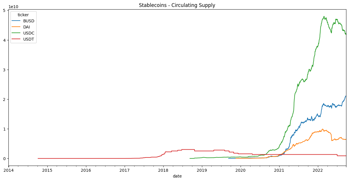
df.unstack().supply_circ.plot(title='Stablecoins - Circulating Supply', figsize=(15,7));

df.unstack().ref_rate_usd.plot(title='Stablecoins - Price', figsize=(15,7));

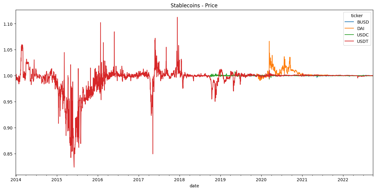
You are now ready to monitor key indicators for stablecoins!

For a deeper dive on how to maximize your use of CryptoDataPy, we explore how to use each one of it’s objects below.

Data Catalog

The DataCatalog allow us to explore what data is available and understand it better.

It includes the following attributes and methods:

• data_sources attribute retrieves information on all the available data sources.

• get_tickers_metadata method retrieves information on available tickers. The get_fields_metadata method retrieves information on available fields.

• search_tickers method allows you to search for tickers by ticker, country, country id, asset class, etc. The search_fields method allows you to search for fields by name, id, category, etc. It also provides identifiers for each data source.

• scrape_stablecoins method scrapes information on stablecoins from the selected source.

To access the data catalog, instantiate a DataCatalog object.

from cryptodatapy.util.datacatalog import DataCatalog 
dc = DataCatalog()

Data Sources

Available data sources

dc.data_sources

{'ccxt': 'https://github.com/ccxt/ccxt',
 'cryptocompare': 'https://min-api.cryptocompare.com/documentation',
 'coinmetrics': 'https://docs.coinmetrics.io/info/markets',
 'glassnode': 'https://glassnode.com/',
 'tiingo': 'https://api.tiingo.com/products/crypto-api',
 'yahoo finance': 'https://finance.yahoo.com/',
 'investpy': 'https://investpy.readthedocs.io/',
 'dbnomics': 'https://db.nomics.world/providers',
 'fred': 'https://fred.stlouisfed.org/'}

Metadata

Available tickers can be accessed with the get_tickers_metadata method.

Note: cryptoasset and individual equity tickers are not listed in the tickers metadata due to a large number of assets. They can be accessed by calling the data source object and using the get_assets_info method to see available tickers.

dc.get_tickers_metadata().head()

	name	description	url	country_id_2	country_id_3	country_name	agg	category	subcategory	mkt_type	frequency	tenor	unit	quote_ccy	tiingo_id	fred_id	dbnomics_id	investpy_id
ticker
ARS	Argentine Peso	Argentine Peso vs. quote currency, spot exchan...	NaN	AR	ARG	Argentina	EM	fx	spot rate	spot	tick	NaN	foreign currency per unit of domestic currrency	NaN	ARS	NaN	NaN	NaN
AUD	Australian Dollar	Australian Dollar vs. quote currency, spot exc...	NaN	AU	AUS	Australia	DM	fx	spot rate	spot	tick	NaN	foreign currency per unit of domestic currrency	NaN	AUD	NaN	NaN	NaN
EUR	Euro	Euro vs. quote currency, spot exchange rate	NaN	AT	AUT	Austria	DM	fx	spot rate	spot	tick	NaN	foreign currency per unit of domestic currrency	NaN	EUR	NaN	NaN	NaN
EUR	Euro	Euro vs. quote currency, spot exchange rate	NaN	BE	BEL	Belgium	DM	fx	spot rate	spot	tick	NaN	foreign currency per unit of domestic currrency	NaN	EUR	NaN	NaN	NaN
BDT	Bangladeshi Taka	Bangladeshi Taka vs. quote currency, spot exch...	NaN	BD	BGD	Bangladesh	NaN	fx	spot rate	spot	tick	NaN	foreign currency per unit of domestic currrency	NaN	BDT	NaN	NaN	NaN

Available fields can be accessed with the get_fields_metadata method.

dc.get_fields_metadata().head()

	name	description	category	subcategory	freq	unit	data_type	cryptocompare_id	coinmetrics_id	ccxt_id	glassnode_id	tiingo_id	investpy_id	dbnomics_id	fred_id	av-daily_id	av-forex-daily_id	yahoo_id
id
date	date	date and time	all	none	all	YYYY-MM-DD-HH:MM:SS	DatetimeIndex	time	time	datetime	t	date	Date	period	DATE	index	index	Date
ticker	ticker symbol	ticker symbol for asset or index	all	none	all	none	string	symbol	market	symbol	NaN	ticker	NaN	NaN	symbol	ticker	ticker	Symbols
bid	best bid price	highest price that a buyer is willing to pay f...	market	quotes	tick	quote currency units	Float64	NaN	bid_price	NaN	NaN	NaN	NaN	NaN	NaN	NaN	NaN	NaN
ask	best ask price	lowest price that a seller is willing to sell ...	market	quotes	tick	quote currency units	Float64	NaN	ask_price	NaN	NaN	NaN	NaN	NaN	NaN	NaN	NaN	NaN
bid_size	bid size	The quantity/size of the highest price bid	market	quotes	tick	asset units	Float64	NaN	bid_size	NaN	NaN	NaN	NaN	NaN	NaN	NaN	NaN	NaN

Search

We can search for tickers with the search_tickers method by column name and keyword.

Let’s look for tickers with assets in the US.

dc.search_tickers(by_col='country_id_2', keyword='US').head()

	name	description	url	country_id_2	country_id_3	country_name	agg	category	subcategory	mkt_type	frequency	tenor	unit	quote_ccy	tiingo_id	fred_id	dbnomics_id	investpy_id
ticker
USD	Us Dollar	Us Dollar vs. quote currency, spot exchange rate	NaN	US	USA	United States	DM	fx	spot rate	spot	tick	NaN	foreign currency per unit of domestic currrency	NaN	USD	NaN	NaN	NaN
USD_TWI	US Dollar Trade-Weighted Index, Nominal Broad	The trade-weighted US dollar index, also known...	https://fred.stlouisfed.org/series/DTWEXBGS	US	USA	United States	DM	fx	index	spot	d	NaN	trade-weighted index	USD	NaN	DTWEXBGS	NaN	NaN
USD_Idx	US Dollar Index Spot	The Ice U.S. Dollar Index (USDX, DXY, DX, or i...	https://www.theice.com/forex/usdx	US	USA	United States	DM	fx	index	spot	tick	NaN	weighted-index	USD	NaN	NaN	NaN	US Dollar Index
USD_Idx_Fut	US Dollar Index Futures, USDX	The Ice U.S. Dollar Index (USDX, DXY, DX, or i...	https://www.theice.com/products/194/US-Dollar-...	US	USA	United States	DM	fx	index	future	tick	NaN	weighted-index	USD	NaN	NaN	NaN	US Dollar Index Futures
USD_Idx_ETF	Invesco DB US Dollar Index Bullish Fund	The Invesco DB US Dollar Index Bullish (Fund) ...	https://www.invesco.com/us/financial-products/...	US	USA	United States	DM	fx	index	etf	tick	NaN	weighted-index	USD	UUP	NaN	NaN	NaN

The same can be done when searching for fields.

For example, let’s look for avaialble on-chain data fields.

dc.search_fields(by_col='category', keyword='on-chain').head()

	name	description	category	subcategory	freq	unit	data_type	cryptocompare_id	coinmetrics_id	ccxt_id	glassnode_id	tiingo_id	investpy_id	dbnomics_id	fred_id	av-daily_id	av-forex-daily_id	yahoo_id
id
add_act	active addresses	number of unique addresses that were active in...	on-chain	addresses	d, w, m, q	addresses	Int64	active_addresses	AdrActCnt	NaN	addresses/active_count	NaN	NaN	NaN	NaN	NaN	NaN	NaN
add_act_new	new addresses	number of new unique addresses that were creat...	on-chain	addresses	d, w, m, q	addresses	Int64	new_addresses	NaN	NaN	addresses/new_non_zero_count	NaN	NaN	NaN	NaN	NaN	NaN	NaN
add_act_sent	active addresses sent	number of unique addresses that were active in...	on-chain	addresses	d, w, m, q	addresses	Int64	NaN	AdrActSentCnt	NaN	addresses/sending_count	NaN	NaN	NaN	NaN	NaN	NaN	NaN
add_act_rec	active addresses received	number of unique addresses that were active in...	on-chain	addresses	d, w, m, q	addresses	Int64	NaN	AdrActRecCnt	NaN	addresses/receiving_count	NaN	NaN	NaN	NaN	NaN	NaN	NaN
add_tot	total address count	number of unique addresses in the network at ...	on-chain	addresses	d, w, m, q	addresses	Int64	unique_addresses_all_time	NaN	NaN	addresses/count	NaN	NaN	NaN	NaN	NaN	NaN	NaN

Stablecoins

We can find static info on stablecoins by using the get_tickers_metadata method and setting the cat parameter to ‘crypto’

dc.get_tickers_metadata(cat='crypto').head()

	name	description	url	country_id_2	country_id_3	country_name	agg	category	subcategory	mkt_type	frequency	tenor	unit	quote_ccy	tiingo_id	fred_id	dbnomics_id	investpy_id
ticker
USDT	Tether USDT	USDT is a cryptocurrency asset issued on the B...	NaN	WL	WLD	World	WL	crypto	stablecoin	spot	tick	NaN	fiat currency per unit of stablecoin	NaN	NaN	NaN	NaN	NaN
USDC	USD Coin	USD Coin (USDC) is a fully collateralized US ...	NaN	WL	WLD	World	WL	crypto	stablecoin	spot	tick	NaN	fiat currency per unit of stablecoin	NaN	NaN	NaN	NaN	NaN
BUSD	Binance USD	Binance USD (BUSD) is a stable coin pegged to ...	NaN	WL	WLD	World	WL	crypto	stablecoin	spot	tick	NaN	fiat currency per unit of stablecoin	NaN	NaN	NaN	NaN	NaN
DAI	Dai DAI	The Maker Protocol, also known as the Multi-Co...	NaN	WL	WLD	World	WL	crypto	stablecoin	spot	tick	NaN	fiat currency per unit of stablecoin	NaN	NaN	NaN	NaN	NaN
FRAX	Frax FRAX	Frax attempts to be the first stablecoin proto...	NaN	WL	WLD	World	WL	crypto	stablecoin	spot	tick	NaN	fiat currency per unit of stablecoin	NaN	NaN	NaN	NaN	NaN

For dynamic/real-time info on stablecoins, we can scrape the data from CoinGecko or CoinMarketCap using the scrape_stablecoins method.

dc.scrape_stablecoins(source='coinmarketcap').head()

	name	price	24h_%_chg	7d_%_chg	mkt_cap	volume_24h	circ_suppkly
ticker
USDT	Tether	1.0000	0.0000	0.0001	6.796102e+10	3.447678e+21	6.795470e+10
USDC	USD Coin	1.0000	0.0001	0.0001	4.959400e+10	3.761719e+19	4.959359e+10
BUSD	Binance USD	0.9996	0.0007	0.0003	2.050853e+10	6.563867e+19	2.051725e+10
DAI	Dai	0.9995	0.0005	0.0001	6.926312e+09	1.957382e+17	6.930064e+09
FRAX	Frax	0.9928	0.0041	0.0055	1.346251e+09	1.413502e+13	1.355966e+09

Data Request

DataRequest provides an intuitive parameter interface which allows you to specify the parameter values for the data you want.

By initializing a DataRequest object, we provide all the relevant parameters needed to retrieve data from the selected data source. DataRequest will automatically convert parameter values to the format required for each data source, allowing the user to experience a consistent and intuitive interface for every data source.

data_req = DataRequest(
    source='cryptocompare',  # provide the name of the supported data source, if not specified defaults to 'CCXT'
    tickers=['btc', 'eth'],  # ticker symbols, if not specified defaults to 'btc'
    freq = 'd',  # frequency of data, if not specified defaults to daily
    quote_ccy = 'USDT',  # quote currency, if not specified defaults to USD/USDT
    exch = None,  # exchance, if not specified defaults to aggregate 
    mkt_type = "spot",  # market type, if not specified defaults to spot
    start_date = None,  # start date, if not specified defaults to beginning of data history
    end_date = None,  # end date, if not specified defaults to end of data history
    fields = ["close", 'volume', "add_act"],  # data fields, if not specified defaults to close
    tz = None,  # timezone, if not specified defaults to 'UTC'
    inst = None,  # institution name, only necessary when retrieving data from institution, e.g. grayscale
    cat = None,  # category of asset or data, must be specified when data source provides data for many asset classes
    trials = 3,  # number of tries when requesting data, defaults to 3 
    pause = 0.1,  # pause between trials to avoid rate limits, defaults to 0.1 sec
    source_tickers = None,  # tickers in data source format, overrides tickers parameter when specified 
    source_freq = None,  # frequency in data source format, overrides tickers parameter when specified 
    source_fields = None,  # fields in data source format, overrides tickers parameter when specified 
           )

print(vars(data_req)) 

{'_source': 'cryptocompare', '_tickers': ['btc', 'eth'], '_frequency': 'd', '_quote_ccy': 'USDT', '_exch': None, '_mkt_type': 'spot', '_start_date': None, '_end_date': None, '_fields': ['close', 'volume', 'add_act'], '_timezone': None, '_inst': None, '_category': None, '_trials': 3, '_pause': 0.1, '_source_tickers': None, '_source_freq': None, '_source_fields': None}

Get Data

GetData retrieves either metadata or time series data from the data source and parameters specified in the data request.

• get_meta method will instantiate a data source object for the selected data source and retrieve all the relevant metadata for it.

• get_series method will retrieve any time series data by initializing the selected data source’s object and using the get_data method. The data is retrieved and wrangled into tidy data format.

Get Meta

Using the DataRequest object we initialized in the previous section, we can get information on availalable assets by using the get_meta method and specifying the metadata method for the data source.

GetData(data_req).get_meta(method='get_assets_info').head()

	Id	Url	ImageUrl	ContentCreatedOn	Name	Symbol	CoinName	FullName	Description	AssetTokenStatus	...	MaxSupply	MktCapPenalty	IsUsedInDefi	IsUsedInNft	PlatformType	AlgorithmType	Difficulty	BuiltOn	SmartContractAddress	DecimalPoints
ticker
42	4321	/coins/42/overview	/media/35650717/42.jpg	1427211129	42	42	42 Coin	42 Coin (42)	Everything about 42 coin is 42 - apart from th...	N/A	...	42	0	0	0	blockchain	scrypt	41.514489	NaN	NaN	NaN
300	749869	/coins/300/overview	/media/27010595/300.png	1517935016	300	300	300 token	300 token (300)	300 token is an ERC20 token. This Token was cr...	N/A	...	300	0	0	0	token	NaN	NaN	ETH	0xaec98a708810414878c3bcdf46aad31ded4a4557	18
365	33639	/coins/365/overview	/media/352070/365.png	1480032918	365	365	365Coin	365Coin (365)	365Coin is a Proof of Work and Proof of Stake ...	N/A	...	-1	0	0	0	blockchain	NaN	NaN	NaN	NaN	NaN
404	21227	/coins/404/overview	/media/35650851/404-300x300.jpg	1466100361	404	404	404Coin	404Coin (404)	404 is a PoW/PoS hybrid cryptocurrency that al...	N/A	...	-1	0	0	0	blockchain	NaN	NaN	NaN	NaN	NaN
433	926547	/coins/433/overview	/media/34836095/433.png	1541597321	433	433	433 Token	433 Token (433)	433 Token is a decentralised soccer platform t...	Finished	...	NaN	NaN	NaN	NaN	NaN	NaN	NaN	NaN	NaN	NaN

5 rows × 36 columns

Get Series

We can then pull the time series data using the get_series method.

df = GetData(data_req).get_series()

df.head()

		close	volume	add_act
date	ticker
2009-01-03	BTC	<NA>	<NA>	1
2009-01-04	BTC	<NA>	<NA>	<NA>
2009-01-05	BTC	<NA>	<NA>	<NA>
2009-01-06	BTC	<NA>	<NA>	<NA>
2009-01-07	BTC	<NA>	<NA>	<NA>

Clean Data

CleanData provides tools for data cleaning.

• OutlierDetection class contains a range of method for outlier detection in time series data. Many traditional outlter detection method are not well suited for time series data.

• Filter class contains methods that allow the filtering of unwanted values (e.g. below a trading liquidity threshold) and tickers (ticker with insufficient price history or stablecoins) to get the data ready for a specific type of analysis (e.g. long/short startegy research, on-chain predictive analytics, etc).

• Impute class deals with missing values in the data with methods that will replace missing values, or repair outliers which were removed by an outlier detection algorithm.

• CleanData class is composed of the previous three classes to allow the creation of a data cleaningn pipeline in a few lines of code.

Outlier Detection

The OutlierDetection class has 8 methods which implement an outlier detection algorithm with the flexibility to set parameters according to use case.

For example, we can use the stl outlier detection method to decompose series into three components: trend, seasonal and residual.

We run it on the dataframe we retrieved in the previous section using the filter_outliers method and show_plot to show the results.

CleanData(df).filter_outliers(od_method='stl', thresh_val=20).show_plot(plot_series=('ETH', 'add_act'))

We can see that it goes a reasonably good job of identifying the large global outliers in active addresses for ETH in late 2017.

Filter

In addition to filtering outliers, the Filter class has several methods allow us to remove data that isn’t of interest to us in our analysis.

For example, let’s say we only want assets with a mimimum of $10 mil USD of average traded volumne, and those with a minimum of 100 price close observations. We can run the filter_avg_trading_val and filter_min_nobs methods on the raw data.

CleanData(df).filter_avg_trading_val(thresh_val=10000000, window_size=30).filter_min_nobs(min_obs=100).show_plot(plot_series=('ETH', 'close'))

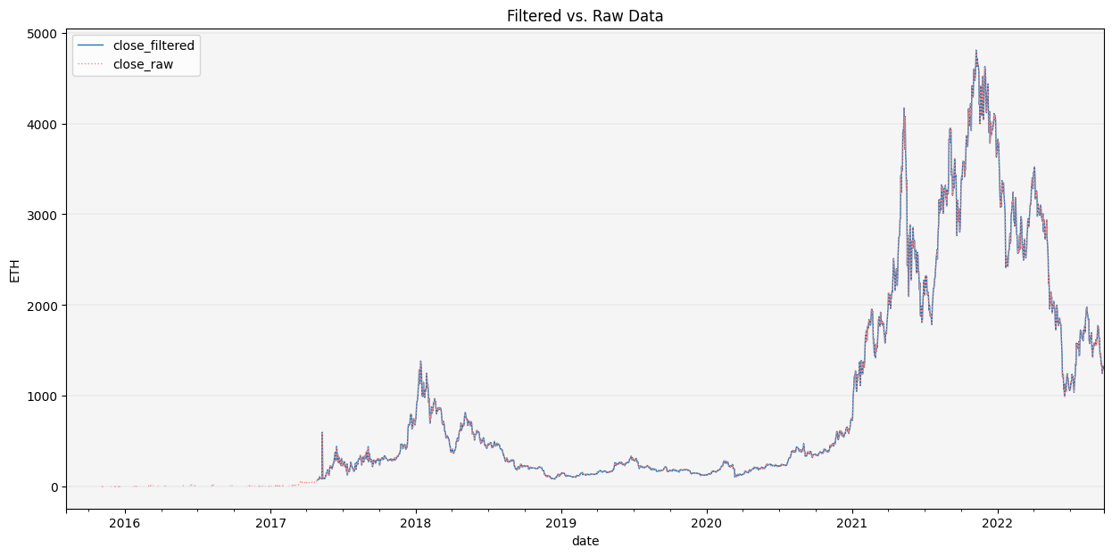
We see that our filter removed values up to early 2017 since ETH didn’t meet the minimum average trading value over a 30-day window.

Impute

The Impute class has several methods that allow us to replace missing values which can cause many issues in predictive/ML models, e.g. scikit-learn and other ML packages may not like missing values and fail to run properly.

We can use it to impute/repair the missing vals/outliers from late 2017 for ETH active addresses with the repair_outliers method.

CleanData(df).filter_outliers(od_method='stl').\
              repair_outliers(imp_method='interpolate').\
              show_plot(plot_series=('ETH', 'add_act'))

Clean Data

CleanData allows us to chain together a series of data cleaning operations and returns either a plot of the filtered vs. raw data, the clean data in a dataframe, the filtered outlies (and forecasts if applicable) and/or a summary of all the data cleaning operations and final data.

CleanData(df).filter_outliers(od_method='stl').\
              repair_outliers(imp_method='interpolate').\
              filter_avg_trading_val(thresh_val=10000000).\
              get(attr='summary')

	close		volume		add_act
	BTC	ETH	BTC	ETH	BTC	ETH
n_obs	2220.00	2198.00	2220.00	2198.00	5004.00	2606.00
%_NaN_start	55.72	56.16	55.72	56.16	0.20	48.03
%_outliers	2.97	2.69	3.65	5.86	5.82	2.01
%_imputed	14.86	8.95	15.46	13.86	5.86	2.03
%_below_avg_trading_val	20.60	11.57	20.52	13.30	64.28	13.46
%_NaN_end	64.44	61.47	64.44	61.47	64.44	61.47

CleanData(df).filter_outliers(od_method='stl').\
              repair_outliers(imp_method='interpolate').\
              filter_avg_trading_val(thresh_val=10000000).\
              get(attr='df')

		close	volume	add_act
date	ticker
2009-01-03	BTC	<NA>	<NA>	<NA>
2009-01-04	BTC	<NA>	<NA>	<NA>
2009-01-05	BTC	<NA>	<NA>	<NA>
2009-01-06	BTC	<NA>	<NA>	<NA>
2009-01-07	BTC	<NA>	<NA>	<NA>
...	...	...	...	...
2022-09-23	ETH	1327.41	2004418.15	501558.0
2022-09-24	BTC	18923.79	330541.25	987921.0
	ETH	1317.25	1068761.99	525728.0
2022-09-25	BTC	18904.56	224299.67	987921.0
	ETH	1292.72	877499.91	525728.0

7621 rows × 3 columns